CONP Portal | Dataset
Numerically Perturbed Structural Connectomes from 100 individuals in the NKI Rockland Dataset
Description:
This dataset contains the derived connectomes, discriminability scores, and classification performance for structural connectomes estimated from a subset of the Nathan Kline Institute Rockland Sample dataset, and is associated with an upcoming manuscript entitled: Numerical Instabilities in Analytical Pipelines Compromise the Reliability of Network Neuroscience. The associated code for this project is publicly available at: https://github.com/gkpapers/2020ImpactOfInstability. For any questions, please contact Gregory Kiar (gkiar07@gmail.com) or Tristan Glatard (tristan.glatard@concordia.ca).
Below is a table of contents describing the contents of this dataset, which is followed by an excerpt from the manuscript pertaining to the contained data.
- impactofinstability_connect_dset25x2x2x20_inputs.h5 : Connectomes derived from 25 subjects, 2 sessions, 2 subsamples, and 20 MCA simulations with input perturbations.
- impactofinstability_connect_dset25x2x2x20_pipeline.h5 : Connectomes derived from 25 subjects, 2 sessions, 2 subsamples, and 20 MCA simulations with pipeline perturbations.
- impactofinstability_discrim_dset25x2x2x20_both.csv : Discriminability scores for each grouping of the 25x2x2x20 dataset.
- impactofinstability_connect+feature_dset100x1x1x20_both.h5 : Connectomes and features derived from 100 subjects, 1 sessions, 1 subsamples, and 20 MCA simulations with both perturbation types.
- impactofinstability_classif_dset100x1x1x20_both.h5 : Classification performance results for the BMI classification task on the 100x1x1x20 dataset.
Dataset
The Nathan Kline Institute Rockland Sample (NKI-RS) dataset [1] contains high-fidelity imaging and phenotypic data from over 1,000 individuals spread across the lifespan. A subset of this dataset was chosen for each experiment to both match sample sizes presented in the original analyses and to minimize the computational burden of performing MCA. The selected subset comprises 100 individuals ranging in age from 6 – 79 with a mean of 36.8 (original: 6 – 81, mean 37.8), 60% female (original: 60%), with 52% having a BMI over 25 (original: 54%).
Each selected individual had at least a single session of both structural T1-weighted (MPRAGE) and diffusion-weighted (DWI) MR imaging data. DWI data was acquired with 137 diffusion directions; more information regarding the acquisition of this dataset can be found in the NKI-RS data release [1].
In addition to the 100 sessions mentioned above, 25 individuals had a second session to be used in a test-retest analysis. Two additional copies of the data for these individuals were generated, including only the odd or even diffusion directions (64 + 9 B0 volumes = 73 in either case). This allows an extra level of stability evaluation to be performed between the levels of MCA and session-level variation.
In total, the dataset is composed of 100 diffusion-downsampled sessions of data originating from 50 acquisitions and 25 individuals for in depth stability analysis, and an additional 100 sessions of full-resolution data from 100 individuals for subsequent analyses.
Processing
The dataset was preprocessed using a standard FSL [2] workflow consisting of eddy-current correction and alignment. The MNI152 atlas was aligned to each session of data, and the resulting transformation was applied to the DKT parcellation [3]. Downsampling the diffusion data took place after preprocessing was performed on full-resolution sessions, ensuring that an additional confound was not introduced in this process when comparing between downsampled sessions. The preprocessing described here was performed once without MCA, and thus is not being evaluated.
Structural connectomes were generated from preprocessed data using two canonical pipelines from Dipy [4]: deterministic and probabilistic. In the deterministic pipeline, a constant solid angle model was used to estimate tensors at each voxel and streamlines were then generated using the EuDX algorithm [5]. In the probabilistic pipeline, a constrained spherical deconvolution model was fit at each voxel and streamlines were generated by iteratively sampling the resulting fiber orientation distributions. In both cases tracking occurred with 8 seeds per 3D voxel and edges were added to the graph based on the location of terminal nodes with weight determined by fiber count.
Perturbations
All connectomes were generated with one reference execution where no perturbation was introduced in the processing. For all other executions, all floating point operations were instrumented with Monte Carlo Arithmetic (MCA) [6] through Verificarlo [7]. MCA simulates the distribution of errors implicit to all instrumented floating point operations (flop).
MCA can be introduced in two places for each flop: before or after evaluation. Performing MCA on the inputs of an operation limits its precision, while performing MCA on the output of an operation highlights round-off errors that may be introduced. The former is referred to as Precision Bounding (PB) and the latter is called Random Rounding (RR).
Using MCA, the execution of a pipeline may be performed many times to produce a distribution of results. Studying the distribution of these results can then lead to insights on the stability of the instrumented tools or functions. To this end, a complete software stack was instrumented with MCA and is made available on GitHub through https://github.com/gkiar/fuzzy.
Both the RR and PB variants of MCA were used independently for all experiments. As was presented in [8], both the degree of instrumentation (i.e. number of affected libraries) and the perturbation mode have an effect on the distribution of observed results. For this work, the RR-MCA was applied across the bulk of the relevant libraries and is referred to as Pipeline Perturbation. In this case the bulk of numerical operations were affected by MCA.
Conversely, the case in which PB-MCA was applied across the operations in a small subset of libraries is here referred to as Input Perturbation. In this case, the inputs to operations within the instrumented libraries (namely, Python and Cython) were perturbed, resulting in less frequent, data-centric perturbations. Alongside the stated theoretical differences, Input Perturbation is considerably less computationally expensive than Pipeline Perturbation.
All perturbations were targeted the least-significant-bit for all data (t=24and t=53in float32 and float64, respectively [7]). Simulations were performed between 10 and 20 times for each pipeline execution, depending on the experiment. A detailed motivation for the number of simulations can be found in [9].
Evaluation
The magnitude and importance of instabilities in pipelines can be considered at a number of analytical levels, namely: the induced variability of derivatives directly, the resulting downstream impact on summary statistics or features, or the ultimate change in analyses or findings. We explore the nature and severity of instabilities through each of these lenses. Unless otherwise stated, all p-values were computed using Wilcoxon signed-rank tests.
Direct Evaluation of the Graphs
The differences between simulated graphs was measured directly through both a direct variance quantification and a comparison to other sources of variance such as individual- and session-level differences.
Quantification of Variability – Graphs, in the form of adjacency matrices, were compared to one another using three metrics: normalized percent deviation, Pearson correlation, and edgewise significant digits. The normalized percent deviation measure, defined in [8], scales the norm of the difference between a simulated graph and the reference execution (that without intentional perturbation) with respect to the norm of the reference graph. The purpose of this comparison is to provide insight on the scale of differences in observed graphs relative to the original signal intensity. A Pearson correlation coefficient was computed in complement to normalized percent deviation to identify the consistency of structure and not just intensity between observed graphs. Finally, the estimated number of significant digits for each edge in the graph was computed. The upper bound on significant digits is 15.7 for 64-bit floating point data.
The percent deviation, correlation, and number of significant digits were each calculated within a single session of data, thereby removing any subject- and session-effects and providing a direct measure of the tool-introduced variability across perturbations. A distribution was formed by aggregating these individual results.
Class-based Variability Evaluation – To gain a concrete understanding of the significance of observed variations we explore the separability of our results with respect to understood sources of variability, such as subject-, session-, and pipeline-level effects. This can be probed through Discriminability [10], a technique similar to ICC which relies on the mean of a ranked distribution of distances between observations belonging to a defined set of classes.
Discriminability can then be interpreted as the probability that an observation belonging to a given class will be more similar to other observations within that class than observations of a different class. It is a measure of reproducibility, and is discussed in detail in [10].
This definition allows for the exploration of deviations across arbitrarily defined classes which in practice can be any of those listed above. We combine this statistic with permutation testing to test hypotheses on whether differences between classes are statistically significant in each of these settings.
With this in mind, three hypotheses were defined. For each setting, we state the alternate hypotheses, the variable(s) which will be used to determine class membership, and the remaining variables which may be sampled when obtaining multiple observations. Each hypothesis was tested independently for each pipeline and perturbation mode, and in every case where it is possible the hypotheses were tested using the reference executions alongside using MCA.
- Individual Variation
HA: Individuals are distinct from one another.
Class definition: Subject ID.
Experiments: Session (1 subsample), Direction (1 subsample), MCA (1 subsample, 1 session). - Session Variation
HA: Sessions within an individual are distinct.
Class definition: Session ID | Subject ID.
Experiments: Subsample, MCA (1 subsample). - Subsample Variation
HA: Direction subsamples within an acquisition are distinct.
Class definition: Subsample | Subject ID, Session ID.
Experiments: MCA.
As a result, we tested 3 hypotheses across 6 MCA experiments and 3 reference experiments on 2 pipelines and 2 perturbation modes, resulting in a total of 30 distinct tests.
Evaluating Graph-Theoretical Metrics
While connectomes may be used directly for some analyses, it is common practice to summarize them with structural measures, which can then be used as lower-dimensional proxies of connectivity in so-called graph-theoretical studies [11]. We explored the stability of several commonly-used univariate (graphwise) and multivariate (nodewise or edgewise) features. The features computed and subsequent methods for comparison in this section were selected to closely match those computed in [12].
Univariate Differences – For each univariate statistic (edge count, mean clustering coefficient, global efficiency, modularity, assortativity, and mean path length) a distribution of values across all perturbations within subjects was observed. A Z-score was computed for each sample with respect to the distribution of feature values within an individual, and the proportion of "classically significant" Z-scores, i.e. corresponding to p < 0.05, was reported and aggregated across all subjects. The number of significant digits contained within an estimate derived from a single subject were calculated and aggregated.
Multivariate Differences – In the case of both nodewise (degree distribution, clustering coefficient, betweenness centrality) and edgewise (weight distribution, connection length) features, the cumulative density functions of their distributions were evaluated over a fixed range and subsequently aggregated across individuals. The number of significant digits for each moment of these distributions (sum, mean, variance, skew, and kurtosis) were calculated across observations within a sample and aggregated.
Evaluating A Complete Analysis
Though each of the above approaches explores the instability of derived connectomes and their features, many modern studies employ modeling or machine-learning approaches, for instance to learn brain-behavior relationships or identify differences across groups. We carried out one such study and explored the instability of its results with respect to the upstream variability of connectomes characterized in the previous sections. We performed the modeling task with a single sampled connectome per individual and repeated this sampling and modelling 20 times. We report the model performance for each sampling of the dataset and summarize its variance.
BMI Classification – Structural changes have been linked to obesity in adolescents and adults [13]. We classified normal-weight and overweight individuals from their structural networks (using for overweight a cutoff of BMI > 25 [14]). We reduced the dimensionality of the connectomes through principal component analysis (PCA), and provided the first N-components to a logistic regression classifier for predicting BMI class membership, similar to methods shown in [14], [15]. The number of components was selected as the minimum set which explained > 90% of the variance when averaged across the training set for each fold within the cross validation of the original graphs; this resulted in a feature of 20 components. We trained the model using k-fold cross validation, with k = 2, 5, 10, and N (equivalent to leave-one-out; LOO).
Dataset README information
Numerically Perturbed Structural Connectomes from 100 individuals in the NKI Rockland Dataset
Crawled from Zenodo
Description
This dataset contains the derived connectomes, discriminability scores, and classification performance for structural connectomes estimated from a subset of the Nathan Kline Institute Rockland Sample dataset, and is associated with an upcoming manuscript entitled: Numerical Instabilities in Analytical Pipelines Compromise the Reliability of Network Neuroscience. The associated code for this project is publicly available at: https://github.com/gkpapers/2020ImpactOfInstability. For any questions, please contact Gregory Kiar (gkiar07@gmail.com) or Tristan Glatard (tristan.glatard@concordia.ca).
Below is a table of contents describing the contents of this dataset, which is followed by an excerpt from the manuscript pertaining to the contained data.
* impactofinstability_connect_dset25x2x2x20_inputs.h5 : Connectomes derived from 25 subjects, 2 sessions, 2 subsamples, and 20 MCA simulations with input perturbations.
* impactofinstability_connect_dset25x2x2x20_pipeline.h5 : Connectomes derived from 25 subjects, 2 sessions, 2 subsamples, and 20 MCA simulations with pipeline perturbations.
* impactofinstability_discrim_dset25x2x2x20_both.csv : Discriminability scores for each grouping of the 25x2x2x20 dataset.
* impactofinstability_connect+feature_dset100x1x1x20_both.h5 : Connectomes and features derived from 100 subjects, 1 sessions, 1 subsamples, and 20 MCA simulations with both perturbation types.
* impactofinstability_classif_dset100x1x1x20_both.h5 : Classification performance results for the BMI classification task on the 100x1x1x20 dataset.
Dataset
The Nathan Kline Institute Rockland Sample (NKI-RS) dataset [1] contains high-fidelity imaging and phenotypic data from over 1,000 individuals spread across the lifespan. A subset of this dataset was chosen for each experiment to both match sample sizes presented in the original analyses and to minimize the computational burden of performing MCA. The selected subset comprises 100 individuals ranging in age from 6 – 79 with a mean of 36.8 (original: 6 – 81, mean 37.8), 60% female (original: 60%), with 52% having a BMI over 25 (original: 54%).
Each selected individual had at least a single session of both structural T1-weighted (MPRAGE) and diffusion-weighted (DWI) MR imaging data. DWI data was acquired with 137 diffusion directions; more information regarding the acquisition of this dataset can be found in the NKI-RS data release [1].
In addition to the 100 sessions mentioned above, 25 individuals had a second session to be used in a test-retest analysis. Two additional copies of the data for these individuals were generated, including only the odd or even diffusion directions (64 + 9 B0 volumes = 73 in either case). This allows an extra level of stability evaluation to be performed between the levels of MCA and session-level variation.
In total, the dataset is composed of 100 diffusion-downsampled sessions of data originating from 50 acquisitions and 25 individuals for in depth stability analysis, and an additional 100 sessions of full-resolution data from 100 individuals for subsequent analyses.
Processing
The dataset was preprocessed using a standard FSL [2] workflow consisting of eddy-current correction and alignment. The MNI152 atlas was aligned to each session of data, and the resulting transformation was applied to the DKT parcellation [3]. Downsampling the diffusion data took place after preprocessing was performed on full-resolution sessions, ensuring that an additional confound was not introduced in this process when comparing between downsampled sessions. The preprocessing described here was performed once without MCA, and thus is not being evaluated.
Structural connectomes were generated from preprocessed data using two canonical pipelines from Dipy [4]: deterministic and probabilistic. In the deterministic pipeline, a constant solid angle model was used to estimate tensors at each voxel and streamlines were then generated using the EuDX algorithm [5]. In the probabilistic pipeline, a constrained spherical deconvolution model was fit at each voxel and streamlines were generated by iteratively sampling the resulting fiber orientation distributions. In both cases tracking occurred with 8 seeds per 3D voxel and edges were added to the graph based on the location of terminal nodes with weight determined by fiber count.
Perturbations
All connectomes were generated with one reference execution where no perturbation was introduced in the processing. For all other executions, all floating point operations were instrumented with Monte Carlo Arithmetic (MCA) [6] through Verificarlo [7]. MCA simulates the distribution of errors implicit to all instrumented floating point operations (flop).
MCA can be introduced in two places for each flop: before or after evaluation. Performing MCA on the inputs of an operation limits its precision, while performing MCA on the output of an operation highlights round-off errors that may be introduced. The former is referred to as Precision Bounding (PB) and the latter is called Random Rounding (RR).
Using MCA, the execution of a pipeline may be performed many times to produce a distribution of results. Studying the distribution of these results can then lead to insights on the stability of the instrumented tools or functions. To this end, a complete software stack was instrumented with MCA and is made available on GitHub through https://github.com/gkiar/fuzzy.
Both the RR and PB variants of MCA were used independently for all experiments. As was presented in [8], both the degree of instrumentation (i.e. number of affected libraries) and the perturbation mode have an effect on the distribution of observed results. For this work, the RR-MCA was applied across the bulk of the relevant libraries and is referred to as Pipeline Perturbation. In this case the bulk of numerical operations were affected by MCA.
Conversely, the case in which PB-MCA was applied across the operations in a small subset of libraries is here referred to as Input Perturbation. In this case, the inputs to operations within the instrumented libraries (namely, Python and Cython) were perturbed, resulting in less frequent, data-centric perturbations. Alongside the stated theoretical differences, Input Perturbation is considerably less computationally expensive than Pipeline Perturbation.
All perturbations were targeted the least-significant-bit for all data (t=24and t=53in float32 and float64, respectively [7]). Simulations were performed between 10 and 20 times for each pipeline execution, depending on the experiment. A detailed motivation for the number of simulations can be found in [9].
Evaluation
The magnitude and importance of instabilities in pipelines can be considered at a number of analytical levels, namely: the induced variability of derivatives directly, the resulting downstream impact on summary statistics or features, or the ultimate change in analyses or findings. We explore the nature and severity of instabilities through each of these lenses. Unless otherwise stated, all p-values were computed using Wilcoxon signed-rank tests.
Direct Evaluation of the Graphs
The differences between simulated graphs was measured directly through both a direct variance quantification and a comparison to other sources of variance such as individual- and session-level differences.
Quantification of Variability – Graphs, in the form of adjacency matrices, were compared to one another using three metrics: normalized percent deviation, Pearson correlation, and edgewise significant digits. The normalized percent deviation measure, defined in [8], scales the norm of the difference between a simulated graph and the reference execution (that without intentional perturbation) with respect to the norm of the reference graph. The purpose of this comparison is to provide insight on the scale of differences in observed graphs relative to the original signal intensity. A Pearson correlation coefficient was computed in complement to normalized percent deviation to identify the consistency of structure and not just intensity between observed graphs. Finally, the estimated number of significant digits for each edge in the graph was computed. The upper bound on significant digits is 15.7 for 64-bit floating point data.
The percent deviation, correlation, and number of significant digits were each calculated within a single session of data, thereby removing any subject- and session-effects and providing a direct measure of the tool-introduced variability across perturbations. A distribution was formed by aggregating these individual results.
Class-based Variability Evaluation – To gain a concrete understanding of the significance of observed variations we explore the separability of our results with respect to understood sources of variability, such as subject-, session-, and pipeline-level effects. This can be probed through Discriminability [10], a technique similar to ICC which relies on the mean of a ranked distribution of distances between observations belonging to a defined set of classes.
Discriminability can then be interpreted as the probability that an observation belonging to a given class will be more similar to other observations within that class than observations of a different class. It is a measure of reproducibility, and is discussed in detail in [10].
This definition allows for the exploration of deviations across arbitrarily defined classes which in practice can be any of those listed above. We combine this statistic with permutation testing to test hypotheses on whether differences between classes are statistically significant in each of these settings.
With this in mind, three hypotheses were defined. For each setting, we state the alternate hypotheses, the variable(s) which will be used to determine class membership, and the remaining variables which may be sampled when obtaining multiple observations. Each hypothesis was tested independently for each pipeline and perturbation mode, and in every case where it is possible the hypotheses were tested using the reference executions alongside using MCA.
1. Individual Variation
HA: Individuals are distinct from one another.
Class definition: Subject ID.
Experiments: Session (1 subsample), Direction (1 subsample), MCA (1 subsample, 1 session).
2. Session Variation
HA: Sessions within an individual are distinct.
Class definition: Session ID | Subject ID.
Experiments: Subsample, MCA (1 subsample).
3. Subsample Variation
HA: Direction subsamples within an acquisition are distinct.
Class definition: Subsample | Subject ID, Session ID.
Experiments: MCA.
As a result, we tested 3 hypotheses across 6 MCA experiments and 3 reference experiments on 2 pipelines and 2 perturbation modes, resulting in a total of 30 distinct tests.
Evaluating Graph-Theoretical Metrics
While connectomes may be used directly for some analyses, it is common practice to summarize them with structural measures, which can then be used as lower-dimensional proxies of connectivity in so-called graph-theoretical studies [11]. We explored the stability of several commonly-used univariate (graphwise) and multivariate (nodewise or edgewise) features. The features computed and subsequent methods for comparison in this section were selected to closely match those computed in [12].
Univariate Differences – For each univariate statistic (edge count, mean clustering coefficient, global efficiency, modularity, assortativity, and mean path length) a distribution of values across all perturbations within subjects was observed. A Z-score was computed for each sample with respect to the distribution of feature values within an individual, and the proportion of "classically significant" Z-scores, i.e. corresponding to p < 0.05, was reported and aggregated across all subjects. The number of significant digits contained within an estimate derived from a single subject were calculated and aggregated.
Multivariate Differences – In the case of both nodewise (degree distribution, clustering coefficient, betweenness centrality) and edgewise (weight distribution, connection length) features, the cumulative density functions of their distributions were evaluated over a fixed range and subsequently aggregated across individuals. The number of significant digits for each moment of these distributions (sum, mean, variance, skew, and kurtosis) were calculated across observations within a sample and aggregated.
Evaluating A Complete Analysis
Though each of the above approaches explores the instability of derived connectomes and their features, many modern studies employ modeling or machine-learning approaches, for instance to learn brain-behavior relationships or identify differences across groups. We carried out one such study and explored the instability of its results with respect to the upstream variability of connectomes characterized in the previous sections. We performed the modeling task with a single sampled connectome per individual and repeated this sampling and modelling 20 times. We report the model performance for each sampling of the dataset and summarize its variance.
BMI Classification – Structural changes have been linked to obesity in adolescents and adults [13]. We classified normal-weight and overweight individuals from their structural networks (using for overweight a cutoff of BMI > 25 [14]). We reduced the dimensionality of the connectomes through principal component analysis (PCA), and provided the first N-components to a logistic regression classifier for predicting BMI class membership, similar to methods shown in [14], [15]. The number of components was selected as the minimum set which explained > 90% of the variance when averaged across the training set for each fold within the cross validation of the original graphs; this resulted in a feature of 20 components. We trained the model using k-fold cross validation, with k = 2, 5, 10, and N (equivalent to leave-one-out; LOO).
Download Using DataLad
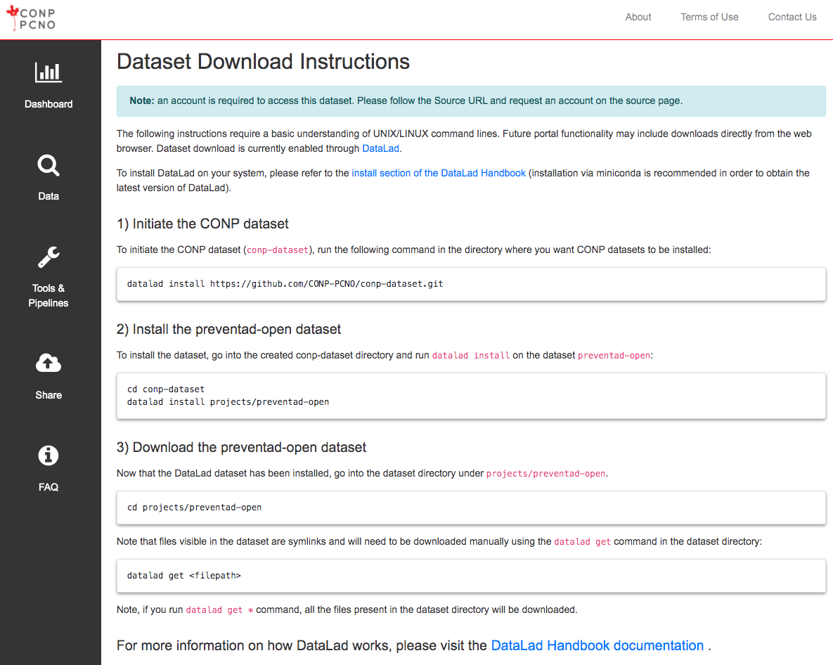
The following instructions require a basic understanding of UNIX/LINUX command lines. Future portal functionality may include downloads directly from the web browser. Dataset download is currently enabled through DataLad.
Note: The conp-dataset requires version >=0.12.5 of DataLad
and version >=8.20200309 of git-annex.
To install DataLad on your system, please refer to the install section of the DataLad Handbook (installation via miniconda is recommended in order to obtain the latest version of DataLad).
1) Initiate the CONP dataset
To initiate the CONP dataset (conp-dataset), run the following
command in the directory where you want CONP datasets to be installed:
datalad install https://github.com/CONP-PCNO/conp-dataset.git
2) Install the Numerically_Perturbed_Structural_Connectomes_from_100_individuals_in_the_NKI_Rockland_Dataset dataset
To install the dataset, go into the created conp-dataset directory and run
datalad install on the dataset Numerically_Perturbed_Structural_Connectomes_from_100_individuals_in_the_NKI_Rockland_Dataset:
cd conp-dataset
datalad install projects/Numerically_Perturbed_Structural_Connectomes_from_100_individuals_in_the_NKI_Rockland_Dataset
3) Download the Numerically_Perturbed_Structural_Connectomes_from_100_individuals_in_the_NKI_Rockland_Dataset dataset
Now that the DataLad dataset has been installed, go into the dataset
directory under projects/Numerically_Perturbed_Structural_Connectomes_from_100_individuals_in_the_NKI_Rockland_Dataset.
cd projects/Numerically_Perturbed_Structural_Connectomes_from_100_individuals_in_the_NKI_Rockland_Dataset
Note that files visible in the dataset are symlinks and will need to be
downloaded manually using the
datalad get
command in the dataset directory:
datalad get <filepath>
Note, if you run datalad get * command, all the files present
in the dataset directory will be downloaded.